
While developing the BVH implementation for Luz, I felt the need to visualize the result of the acceleration structure in its full three-dimensional glory. Debugging this acceleration structure can be cumbersome and spotting errors simply by investigating the code isn’t enough. In fact, an incorrectly implemented BVH can still yield good performance which is why it’s so tricky to notice it just by inspecting the recorded performance impact of each frame. Indeed, a good raytracer should provide analytics but we could be tricked by our own data in this case, which is why need to combine our analytics with a visual model of the acceleration structure.
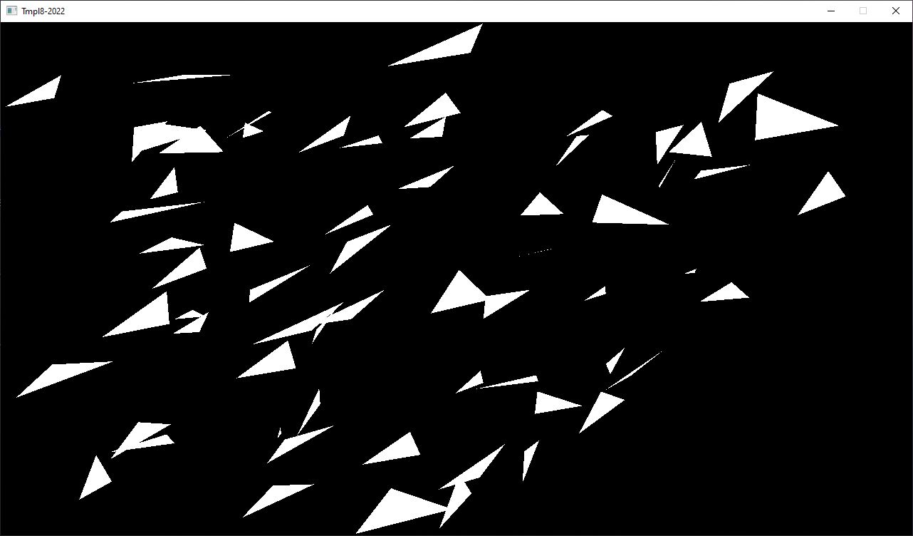
I should note that my demonstration here today is heavily influenced by Jacco Biker, who wrote potentially one of the greatest tutorials on the subject earlier this year, go have a look if you are interested in finding out more here. In this first step of his BVH implementation, Jacco generates a scene of 64 randomly scattered triangles and traces them using the classic Möller-Trumbore algorithm.
I could start on implementing a bounding box visualizer directly in Luz but that would take the focus away from actual implementation of the BVH algorithm, which is more of a priority at this stage of the Luz development. When the BVH acceleration structure has been built, I have an array of nodes consisting of the min and max points produced from tightly fitting them to the primitives and recursively splitting each node until optimal boundaries have been found. These bounding boxes can easily be visualized in Blender, so I went ahead and exported them.
1. Write out each AABB min and max point to file
// -----------------------------------------------------------
// HEADER
// -----------------------------------------------------------

__declspec(align(32)) struct BvhNode
{
    float3 aabbMin, aabbMax; //24 bytes
    uint leftFirst, triCount; //8 bytes
    bool isLeaf() { return triCount > 0; }
};

// Middle-hand struct for writing float3 data
struct point
{
    float x, y, z;
};

#define N 64
BvhNode bvhNode[N * 2 - 1];

// -----------------------------------------------------------
// OUTPUT
// -----------------------------------------------------------

std::ofstream bvhFile("bvh.pts", std::ios::out | std::ios::binary);
const unsigned int numNodes = N * 2 - 1;
for (unsigned int i = 0; i < numNodes; ++i)
{
   const float3& fMin = bvhNode[i].aabbMin;
   const float3& fMax = bvhNode[i].aabbMax;

   const point min = { fMin[0], fMin[1], fMin[2] };
   bvhFile.write((char*)&min, sizeof(point));

   const point max = { fMax[0], fMax[1], fMax[2] };
   bvhFile.write((char*)&max, sizeof(point));
}
2. Read two float3 at a time from the imported float3 data array, interpret them as vertices and use them as input to a mesh object
import bpy
import bmesh
import struct

bvhFile = open("bvh.pts", "rb")
N = 64
numNodes = N * 2 - 1

for i in range(numNodes):
    minPoint = struct.unpack('3f', bvhFile.read(12))
    maxPoint = struct.unpack('3f', bvhFile.read(12))

    aabbToMesh(minPoint, maxPoint)
3. Create a box from the mesh vertices and set the display type to bounding box
def aabbToMesh(min, max):
    """
    Creates mesh from AABB min and max points displayed as bounding box
    Parameters:
        min - minimum point in AABB
        max - maximum point in AABB
    """

    verts = [(min[0], min[1], min[2]), (max[0], max[1], max[2])]
    mesh = bpy.data.meshes.new("mesh")
    obj = bpy.data.objects.new("Node", mesh)

    scene = bpy.context.collection
    scene.objects.link(obj)
    bpy.context.view_layer.objects.active = obj
    bpy.context.object.display_type = 'BOUNDS'
    bpy.context.active_object.select_set(state=True)

    mesh = bpy.context.object.data
    bm = bmesh.new()

    for v in verts:
        bm.verts.new(v)

    bm.to_mesh(mesh)
    bm.free()
After we have completed these steps, this is the resulting model. Already it’s easier to get an idea how the structure partitions the scene but without the primitives, we don’t have the full picture of what’s going on here yet.
Just like the bounding box points, we can output these to a file and import them as a final step. A quick way to export the triangles from the raytracing application is to use the STL format, which can be seen below. For this demonstration, I will only be using flat shading so we can skip the normals of the primitives.
solid Triangles_output
  facet normal 0 0 0
    outer loop
      vertex -2.46422 -4.2492 -0.232984
      vertex -2.30149 -3.81082 0.273664
      vertex -1.63817 -3.4793 0.30526
    endloop
  endfacet
endsolid
Of course, there will be plenty more triangles in the actual file but you get the idea. With the STL file written, we can now import it to Blender and see the full picture of the structure:
In summary, this was the quickest way I could think out to visualize the BVH acceleration structure when I started implementing it for Luz. Over time, this will be integrated as a separate feature into Luz once my implementation has been proved to work for more complicated scenes than just a few single textured meshes as demonstrated in my alpha demo video from last month.
Live long and prosper!


