In the spring of 2025, I created two short demo songs for my music project “Khazar Eli” for which I also painted a cover.
KHAZAR ELI – Music Project Demo

Software Developer
In the spring of 2025, I created two short demo songs for my music project “Khazar Eli” for which I also painted a cover.

Back again with a small vacation project!
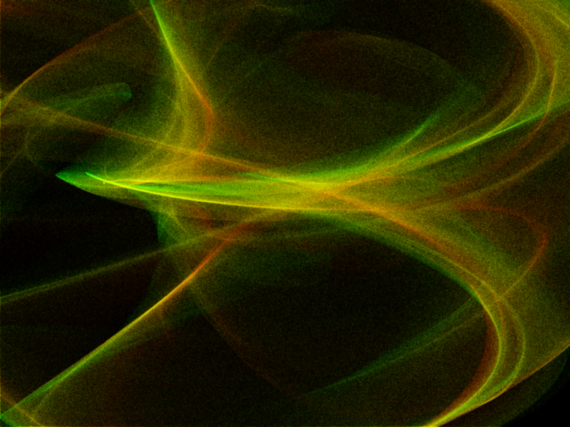
Since I just learned to play most parts of the song Stinkfist and recorded it in one of my sessions, I wanted to accompany that with a short animation in true TOOL fashion. This was a quick effect I threw together but I thought it would be fun just to cover some of the highlights in the process.
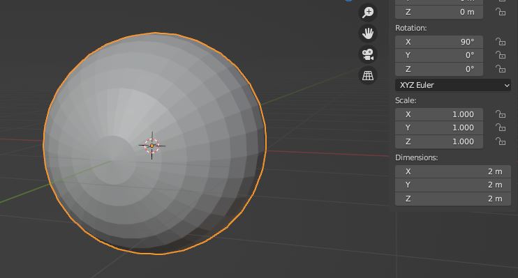
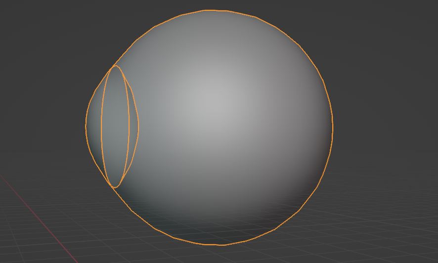
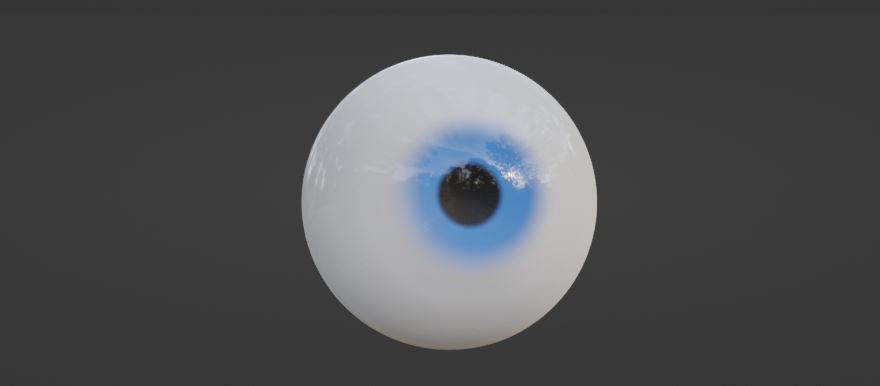
The UV sphere is a good starting mesh but we have to remember that eyes aren’t perfectly round so we need to take that into account. The edges at the pole create rendering artifacts as well, so I remove its geometry and insert another sphere to use as reference when I’m scaling a subdivided surface onto the opening of the eye. Then the backfaces inside of that reference sphere can be be positioned appropriately to function as the iris.
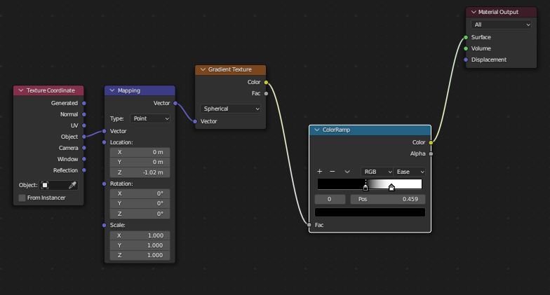
Making procedural eyes in Blender relies heavily on the usage of spherical gradient maps, in which you create masks to form the iris and its various color gradients. The masks are also used to turn off any other effects that overlap with the iris, such as blood vessels which can be created using Voronoi texture nodes.
https://docs.blender.org/manual/en/latest/render/shader_nodes/textures/voronoi.html
Just to give you an idea of the underlying shader pipeline, this is what it will look like for most of the time. Lots of masks stacked on top of each other and mixed to combine various effects.
Note that in order to actually be able to make it transparent, we have to enable screen space refractions in the material properties or otherwise this approach won’t work.
From here on, I start modelling an eye socket using the reference image and make sure I’ll capture the general shape of the grooves since they are an important detail.

I let Blender solve the UV-mapping for me and I barely had to make any adjustment to the automatic unwrap, this is a nice thing with open meshes that are only viewed from one direction. With the model for the eye socket ready, I’m going to project the original image onto the mesh to get my final texture. Here I’m also starting to make use of the Voronoi Texture to simulate the pigmented layer at the front of our eyes.
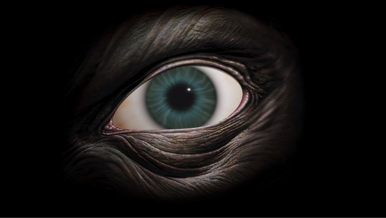
On top of this, I also mix in some of the original iris from the painting.
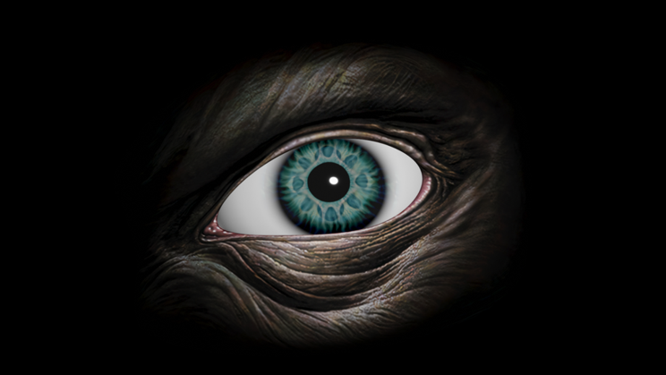
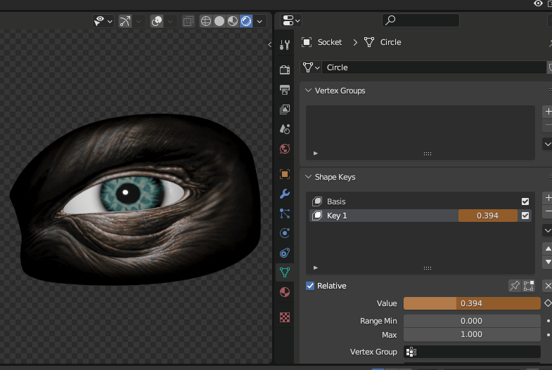
To give the eye a bit more life, I’m going to insert a small amount of morphing on the eyelids using a shape key.
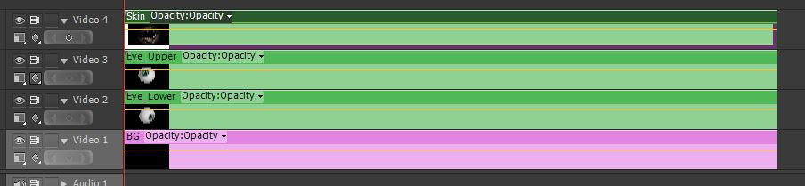
In order to overlap the eyes with as little visual artifacts as possible, I essentially split up each mesh into its separate rendering layer and made a composition of them later in Adobe Premiere.
I settled for a gentle swaying pattern for the camera to make it a bit more haunting and a bit of noise to set the mood, it also helped to blur out the edges of the mesh.
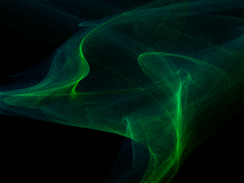
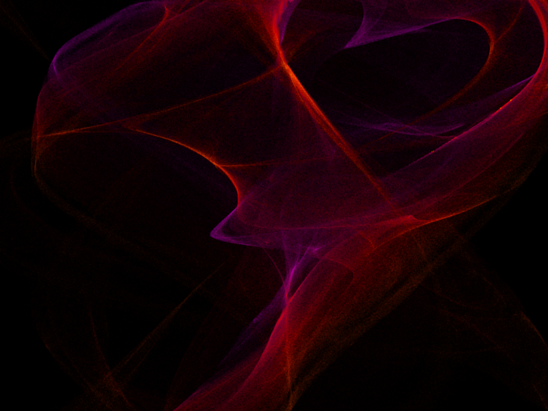
Below you can see the rendered sequence that I used for my Stinkfist cover, I don’t know about my guitar techniques but I had a lot of fun doing this. I’m thinking about turning this into a series and make a new effect for each TOOL song I learn but that’s yet to come.

Table Of Contents
Long time no see!
Today I’m going to return to the subject of attractors which I started exploring a while back on this page and see if I can come up with some new implementations that I haven’t tried out before. If you want to read about my initial exploration of the Clifford Attractors, you can find it here: Luz: Clifford Attractors Plugin
The reason I was drawn to attractors in the first place is that with a relatively small effort, you can come up with an amazing piece of abstract art that takes on a life of its own in front of your eyes. I will use Unreal Engine 5 to demonstrate how an attractor system can be implemented in Niagara and also expanded to allow the implementation of different attractor solutions.
Besides being algebraically represented, strange attractors can be treated like just any other particle system (a physical system) where we have starting conditions and a system that evolves over time.
There are many mathematical explanations to what attractors are but the most straightforward way to look at it (the way I look at it I should say) is points within a shape or region that is being pulled around by a set of initial conditions and the systems acting upon these conditions. When I say system, I refer to the system of equations that simulates the behaviors of natural phenomena such as weather. These equations are non-linear, meaning they don’t have a predictable outcome and therefore these attractors falls into the subject of “chaos theory”. For example, two points on the attractor that are near each other at one time can be far apart at later times, resulting in various trajectories.
So if you’ve ever stopped and witnessed a whirlwind of leaves in the fall circling in various patterns, or perhaps observed clouds taking on different formations over time when you’re lying in the grass on a warm summer day, this is essentially the same what we are trying to accomplish with attractors. Fittingly, the first example of a strange attractor was the Lorenz attractor which is based in a mathematical model of the atmosphere. So these behaviors that I mentioned, they are often determined by natural laws such as the laws of fluid dynamics, which is the case for the Lorenz attractor.
What does this mean for us as visual artists? Well, we can utilize these concepts to follow the trajectories of the points in the system and visualize them with shaders! The implementation we are making today is a Dequan Li attractor, which is a modification of the Lorenz system.
For this implementation, we want to start out with a complete blank scene.
File > New Level > Empty Level
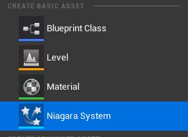
Next, we need to create a Niagara system.
Right-click in the workspace > Create Basic Asset> Niagara System
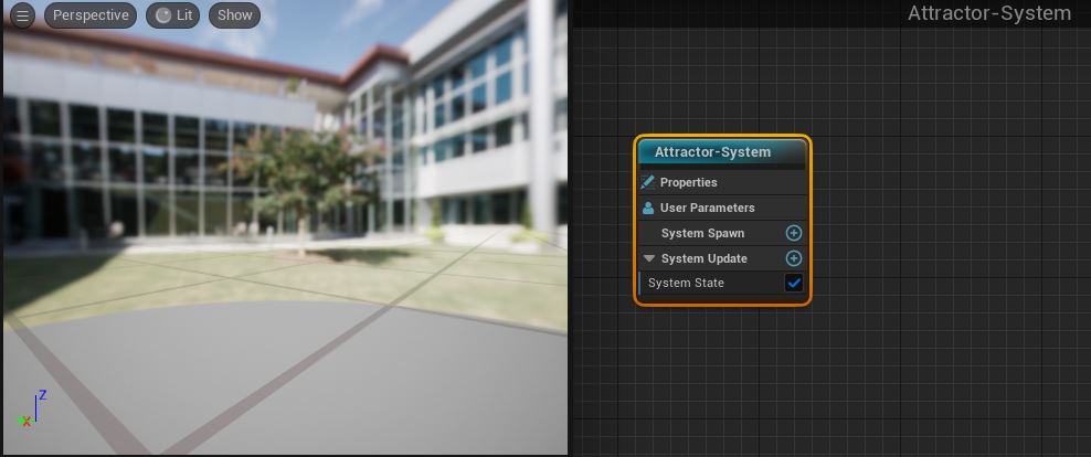
When we double-click the Niagara System we created, we will open up the editor for the simulation.
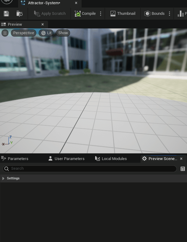
The environment background will be somewhat distracting so in order to remove it, you must head over the the preview settings in the Windows tab.
Window > Preview Scene Settings > Environment > Show Environment
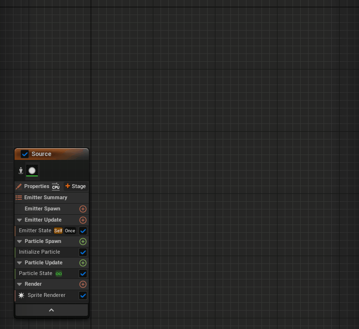
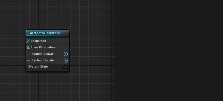
To start off our implementation, create a new empty emitter which we are going to use as our “source” for the system
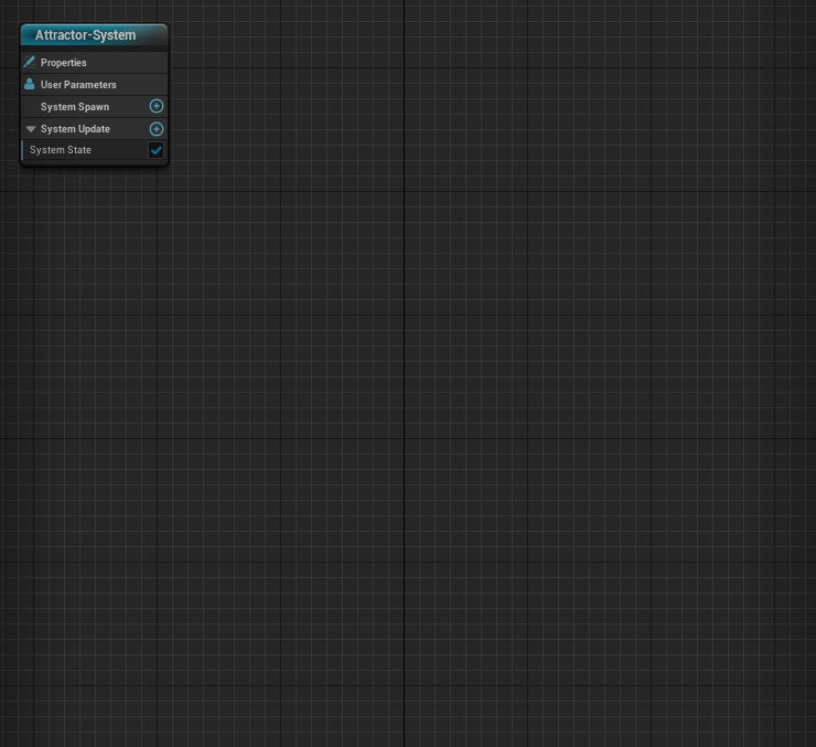
Turn on local space for the emitter and set the loop duration mode to infinite. Local space makes sure that the particles spawned by this emitter is relative to the emitter origin.
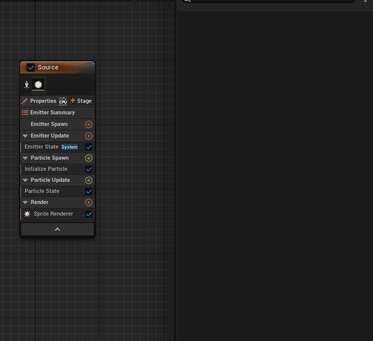
Loop the particle lifetime in the particle state
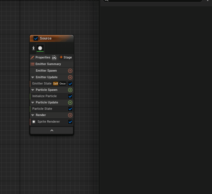
Add a scratch pad module to the particle state, which we will use to implement the main logic of the particle update
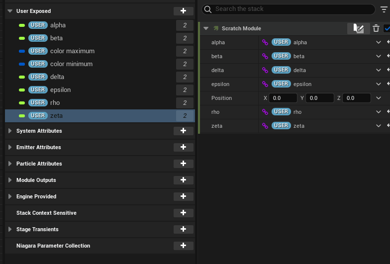
With the scratch pad module, we’re approaching it like a regular shader pipeline where we will gather inputs in the form of a buffer (Map Get node). In the Map Get node, we will create float variables for the different constants that are commonly found in the equations.
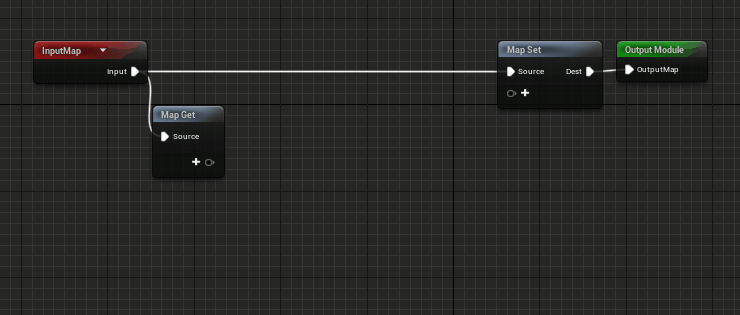
We also create a position variable which we will later on feed with the current position of each particle.

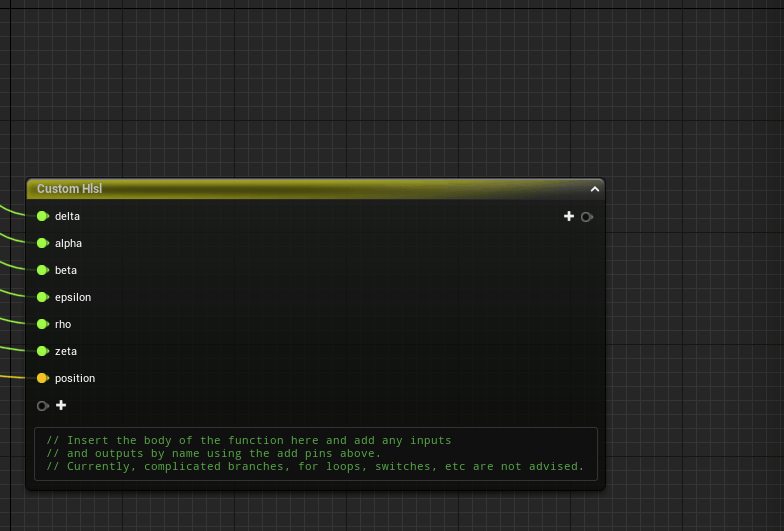
Next we create an custom HLSL node (High-level shader language) which we will attach our inputs to and also define the output.
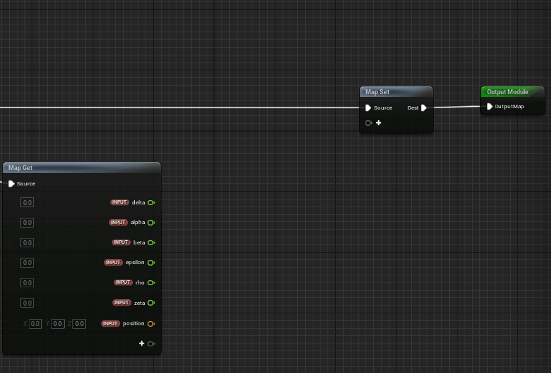
The output from this stage will be the new position of the particle and this will be directed to the “Velocity” attribute of particle system.
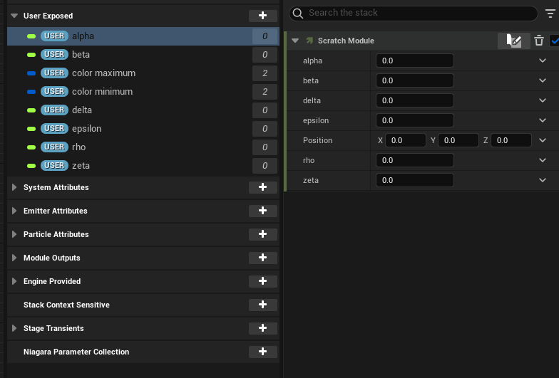
Before we get into writing the shader, I’m going to hook up the input parameters to the shader with user defined fields so that we can quickly change the constants from the main editor without having to open the particle system every time we want to change them.
Next one is important because now we must direct the particle position to the shader “position” input parameter, otherwise we won’t be able to modify the particle position.
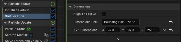
To actually make the particles appear, we need to add “Spawn Particles in Grid” underneath the “Emitter Update”.
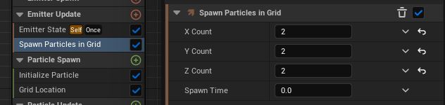
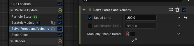
If you ever need to constrain the speed of your particles and I would recommend having this on regardless, you can control this in “Solve Forces and Velocity” underneath the “Particle Update” category.
We can also setup a color range in the “Particle Spawn” category using our exposed user variables to give the attractor a gradient look. With the sprite render enabled as well, we can also expose control of the sprite size.
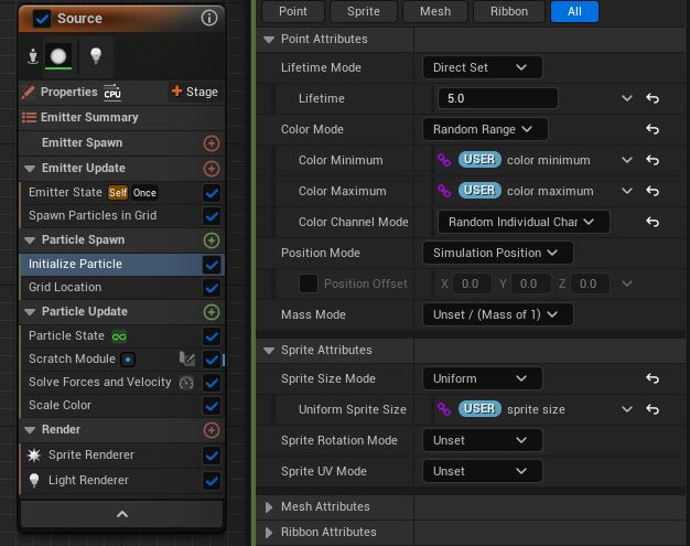
Also, make sure to set an appropriate boundary between the particles in order to not have them bleed into each other.
From here on, it’s possible to use this emitter as a base for other emitters by allowing them to sample the “Source” emitter and extend its behaviors, or even attach additional rendering options onto it. As you can see below, I have chained together the particle system with two renderers; one sprite renderer attached on the “Source” emitter and a ribbon renderer attached onto a second emitter.
There is a final detail I would like to mention that is useful when exporting rendered sequences of particle systems in Unreal Engine and that is utilizing the warmup settings in the particle system properties. Depending on how you want to capture your particle system, whether it is using an orbital camera or a custom defined path, it might take some time before the attractor has evolved enough so that the points are separated enough that it will fill up most of the frame. In order to not waste any frames and skip forward into the simulation, we set a warmup timer in seconds.
You might only notice this effect in the preview window of your particle system but you will also see this in effect when you are rendering the sequence if you’ve added warmup frames in your render config as well. I’m not certain why this option is hidden underneath the “Anti-Aliasing” setting but there you have it.
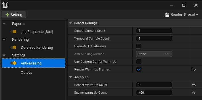
During export, you will see this status in the lower right corner indicating that the engine is still warming up. Once the amount of frames that were specified has been reached, the renderer will start to export the images to disk.

With all those preparations made, we can now translate the Dequan Li equations to a HLSL shader code below:
out_position = position;
float x = position.x;
float y = position.y;
float z = position.z;

float dx = alpha * (y-x) + delta * x * z;
float dy = rho * x + zeta * y - x * z;
float dz = beta * z + x * y - epsilon * pow(x, 2);

out_position += vec3(dx, dy, dz);
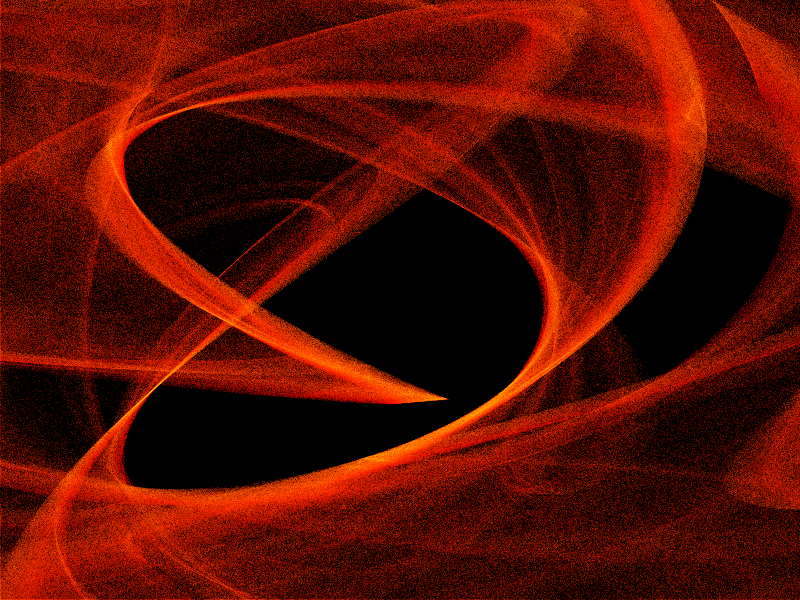
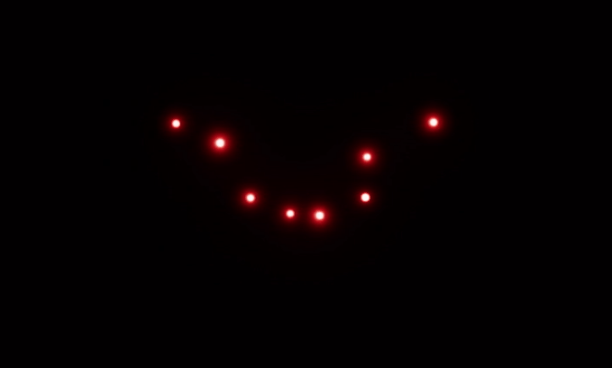
This was a quick overview of how the Niagara system in Unreal Engine 5 can be used to visualize strange attractors using a HLSL shader approach. Below you can see the rendered sequence in action where I have used a scaled up Dequan Li attractor that I produced for this post:

Shadertoy.com is an online community and tool for creating and sharing shaders through WebGL, used for both learning and teaching 3D computer graphics in a web browser.
The approach in Shadertoy is to produce images with minimal data input to the graphics pipeline where most of the heavy lifting is performed directly in the fragment shader. The vertex shader in this case is only used to process a full-screen quad which functions as the canvas for these visual effects. This is not always the most ideal way of doing 3D-programming but if you want to play around with a lot of math and get creative, you’ve come to the right place.
In this post, I summarize the discoveries I’ve made along the way and updates to Luz that were necessary to implement Shadertoy support.
Here is a demo with a couple of shaders from Shadertoy that this plugin can interpret and render using Luz. They are all listed below in order, all rights belong to their respective owners:
As you can see, many shaders written for Shadertoy features input support and this data had not yet been forwarded to previous plugins. Alongside with mouse position updates, input callbacks within Luz are now also forwarded to the plugins. This enables us to create interactive turntable cameras or move the position of the camera.
If you have a DLL that links to dependencies from the same folder, such as other dynamic link libraries, then it’s necessary to add that DLL directory before attempting to call LoadLibrary. Otherwise you will be given the error code 126 from GetLastError, which translates to ERROR_MOD_NOT_FOUND. This could be somewhat misleading at first if your targeted DLL file does exist at the specified location, but it’s in fact the dependency of the plugin that cannot be found.
const size_t pos = path.find_last_of("\\");
SetDllDirectory(path.substr(0, pos).c_str());

pluginHinstance = ::LoadLibrary(path.c_str());
This is an easy mistake to make and I was naive to think that LoadLibrary would be able to resolve this on its own by looking in the same folder the DLL was loaded from. I found the following statement from the official documentation which gave me a better understanding of the issue:
If a DLL has dependencies, the system searches for the dependent DLLs as if they were loaded with just their module names. This is true even if the first DLL was loaded by specifying a full path.
Hence, this is why we need to make the call to SetDllDirectory.
Unlike Vulkan where headless rendering is possible, OpenGL requires a window to create the context. It’s not really a problem since we can specify to GLFW to create the window as hidden so we will never be able to interact with it. Once we have set it up, we only need the window to swap buffers between render calls.
glfwWindowHint(GLFW_VISIBLE, GLFW_FALSE);
window = glfwCreateWindow(width, height, title, monitor, NULL);
Since OpenGL also defines bottom left corner of the screen as (0, 0) unlike in other API:s where (0,0) is located in the upper left corner of the screen, I felt the need to provide a way to compensate for this without tying myself up to any API conventions. Luckily, ImGui::Image lets me provide the coordinates for the corners of the image and I decided to let the user define what positions the corners should be. This means we can render an image as usual regardless of the convention used by the underlying API in the plugin and then Luz compensates it for final presentation.
  "Framebuffer": {
	"UV0": {"x": 0.0, "y": 1.0 },
	"UV1": {"x": 1.0, "y": 0.0 }
  },
Before I started writing the Shadertoy plugin, Luz had no concept of criticality levels in terms of return values from the various stages of execution. If something failed in the plugin, Luz would unload the plugin and return the latest error message.
In this case when you’re reloading shaders on the fly, it’s only a matter of time before you slip and accidentally write some invalid syntax (it’s kind of the whole point to allow for experimentation). Just because a shader could not be compiled, I don’t want Luz to unload the plugin but rather just print the latest error message and keep the plugin active. So it was about time that I introduced some criticality levels:
While the criticality levels themselves don’t always guarantee proper error handling, it can be a guiding tool for troubleshooting along with the messages recorded in the log. Below is an example of how the color coding looks like in the log:
In order to reach full compatibility with Shadertoy, my plugin will have to increase its number of iChannel uniforms to a total of four. They are currently only interpreted as sampler2D uniforms but since I’m looking to support cube maps as well, I will work on adding samplerCube uniforms for the next version. Another concept in Shadertoy that I haven’t implemented yet are buffer stages which can serve as input into any of the four iChannel slots to allow for more advanced and longer chains of computations.

Today I’ve been diving into the works of Clifford A. Pickover after reading some of his early books on computer graphics when I stumbled over the Clifford Attractor on Paul Bourke’s homepage.
These chaotic attractors can produce stunning visualizations and with example code provided by Paul Richards, I was able to write a plugin for Luz that could render them in real-time. Paul Bourke goes into more detail further down in the page about how these color effects are achieved:
The main thing happening here is that I don’t draw the attractor to the final image. Rather I create a large grid of 32 bit (int or float) and instead of drawing into that in colour I evaluate points on the attractor and just increment each cell of the grid if the attractor passes through it.
So it’s essentially a 2D histogram for occupancy. One wants to evaluate the attractor much more/longer than normal in order to create a reasonable dynamic range and ultimately smooth colour gradients. I then save this 2D grid, the process of applying smooth colour gradients comes as a secondary process … better than trying to encode the right colour during the generation process. One can even just save the grid as a 16 or 32 bit raw, open in PhotoShop and apply custom gradient maps there.
Of course this is “just” a density mapping of the histogram and doesn’t immediately allow for colouring based upon other attributes of the attractor path, such as curvature. But such attributes can be encoded into the histogram encoding, for example the amount added to a cell being a function of curvature.
Alongside playing around with the Clifford Attractor, I’ve added a couple of minor features to Luz:
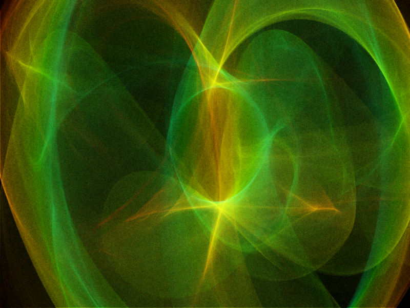
Here is a presentation of the Clifford Attractors I rendered during my session, they are somewhat grainy but the result is nevertheless pleasing to look at.
Until next time, have a good weekend!

Back again with another update on my experimental renderer Luz, which I’ve made some drastic changes to over the last couple of months. This change in design came from the idea of turning Luz into a stand-alone viewport application in which plugins can be loaded to write to the Luz viewport using various CPU or GPU based rendering approaches.
Here is a showcase of the first successfully developed plugin using Vulkan for Luz. When it comes to prototyping, it’s back to the holy triangle. Nothing more, nothing less.
Instead of focusing on raytracing, Luz now supports a wide range of plugins to be developed that can be viewed and analyzed within its viewport. Plugins are loaded into Luz at runtime and can draw into the framebuffer allocated by Luz. With this “black box” approach for viewing the final image of a render call, window handling can be reused across different plugins and the developer (me) can fully focus on developing the 3D-techniques without having to reinvent the wheel by making new window handling systems for each project.
A plugin is a dynamic-link library underneath the surface and to make this work in practice, both Luz and the plugin shares the same interface. Only two functions are necessary at the moment for the plugin model: “GetInterface” and “FreeInterface”. Since plugins might have different usages, I’ve allowed for there to be different interfaces in case the standard protocol lacks the necessary flexibility.
#ifndef TRIANGLES_INTERFACE_H
#define TRIANGLES_INTERFACE_H

#include "Interfaces/VulkanPluginInterface.h"

extern "C"
{
    bool GetPluginInterface(VulkanPluginInterface** pInterface);
    typedef bool(*GETINTERFACE)(VulkanPluginInterface** pInterface);

    bool FreePluginInterface(VulkanPluginInterface** pInterface);
    typedef bool(*FREEINTERFACE)(VulkanPluginInterface** pInterface);
}

#endif
One important detail to mention here is that both the plugin and Luz needs to use the same CRT in order to share the same heap, in case they require knowledge of allocated resources on each side of the boundary. If they don’t match, you can end up having some heap validation errors that don’t make a whole lot of sense, simply because the addresses acquired won’t match. Another rule I have enforced is that neither the plugin or the application allocates dynamic memory within each others domain. Once the interface has been established between the plugin and Luz, we can access the following functions below:
#ifndef PLUGIN_INTERFACES_I_VULKAN_PLUGIN_H
#define PLUGIN_INTERFACES_I_VULKAN_PLUGIN_H

struct VulkanPluginInterface
{
	virtual bool initialize() = 0;
	virtual bool release() = 0;
	virtual bool execute() = 0;
	virtual bool reset() = 0;

	virtual bool getImageData(void* pBuffer, const unsigned int width, const unsigned int height) = 0;

	virtual bool sendData(const char* label, void* data) = 0;

	virtual float getLastRenderTime() = 0;

	virtual const char* getLastErrorMsg() = 0;

	virtual const char* getPluginName() = 0;
};

#endif
Each plugin is also accompanied by a JSON based .ui file where UI elements can be specified. Input fields, scalars, checkboxes, headers and many more ImGui elements can be specified here to customize the controls exposed by the plugin to modify its behavior. Each interaction with the UI elements in Luz is then sent back to the plugin using events and these are mapped against the contents of the .ui file so the plugin will always knows which UI elements received updates.
{
  "Document" : {
    "Description" : "Vulkan Plugin Configuration"
  },
  "Framebuffer": {
	"Resolutions": "800x600,1024x768",
	"Modes": "Interactive",
	"Hardware": "GPU",
	"Methods": "Copy",
	"SupportMultithreading": true,
	"DataFormat": "Byte"
  },
  "Menu" : {
	"Elements": [
	  { "Type": "BeginHeader", "Title": "Pipeline" },
		{ "Type": "FloatScalar", "Title": "Rotation Factor" },
	    { "Type": "Tick", "Title": "Backface Culling", "Reset": true },
	    { "Type": "Dropdown", "Title": "Polygon Mode", "Args": "Fill,Line", "Reset": true },
	  { "Type": "EndHeader" }
	]
  }
}
Hope you’ve enjoyed this demo, I’ll be back again in the near future with more demos and features added to Luz 🙂

While developing the BVH implementation for Luz, I felt the need to visualize the result of the acceleration structure in its full three-dimensional glory. Debugging this acceleration structure can be cumbersome and spotting errors simply by investigating the code isn’t enough. In fact, an incorrectly implemented BVH can still yield good performance which is why it’s so tricky to notice it just by inspecting the recorded performance impact of each frame. Indeed, a good raytracer should provide analytics but we could be tricked by our own data in this case, which is why need to combine our analytics with a visual model of the acceleration structure.
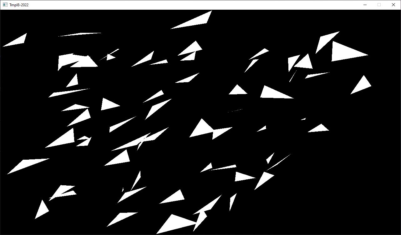
I should note that my demonstration here today is heavily influenced by Jacco Biker, who wrote potentially one of the greatest tutorials on the subject earlier this year, go have a look if you are interested in finding out more here. In this first step of his BVH implementation, Jacco generates a scene of 64 randomly scattered triangles and traces them using the classic Möller-Trumbore algorithm.
I could start on implementing a bounding box visualizer directly in Luz but that would take the focus away from actual implementation of the BVH algorithm, which is more of a priority at this stage of the Luz development. When the BVH acceleration structure has been built, I have an array of nodes consisting of the min and max points produced from tightly fitting them to the primitives and recursively splitting each node until optimal boundaries have been found. These bounding boxes can easily be visualized in Blender, so I went ahead and exported them.
1. Write out each AABB min and max point to file
// -----------------------------------------------------------
// HEADER
// -----------------------------------------------------------

__declspec(align(32)) struct BvhNode
{
    float3 aabbMin, aabbMax; //24 bytes
    uint leftFirst, triCount; //8 bytes
    bool isLeaf() { return triCount > 0; }
};

// Middle-hand struct for writing float3 data
struct point
{
    float x, y, z;
};

#define N 64
BvhNode bvhNode[N * 2 - 1];

// -----------------------------------------------------------
// OUTPUT
// -----------------------------------------------------------

std::ofstream bvhFile("bvh.pts", std::ios::out | std::ios::binary);
const unsigned int numNodes = N * 2 - 1;
for (unsigned int i = 0; i < numNodes; ++i)
{
   const float3& fMin = bvhNode[i].aabbMin;
   const float3& fMax = bvhNode[i].aabbMax;

   const point min = { fMin[0], fMin[1], fMin[2] };
   bvhFile.write((char*)&min, sizeof(point));

   const point max = { fMax[0], fMax[1], fMax[2] };
   bvhFile.write((char*)&max, sizeof(point));
}
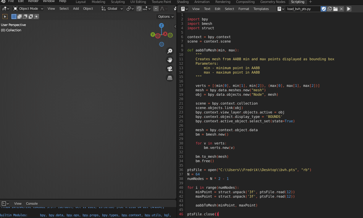
2. Read two float3 at a time from the imported float3 data array, interpret them as vertices and use them as input to a mesh object
import bpy
import bmesh
import struct

bvhFile = open("bvh.pts", "rb")
N = 64
numNodes = N * 2 - 1

for i in range(numNodes):
    minPoint = struct.unpack('3f', bvhFile.read(12))
    maxPoint = struct.unpack('3f', bvhFile.read(12))

    aabbToMesh(minPoint, maxPoint)
3. Create a box from the mesh vertices and set the display type to bounding box
def aabbToMesh(min, max):
    """
    Creates mesh from AABB min and max points displayed as bounding box
    Parameters:
        min - minimum point in AABB
        max - maximum point in AABB
    """

    verts = [(min[0], min[1], min[2]), (max[0], max[1], max[2])]
    mesh = bpy.data.meshes.new("mesh")
    obj = bpy.data.objects.new("Node", mesh)

    scene = bpy.context.collection
    scene.objects.link(obj)
    bpy.context.view_layer.objects.active = obj
    bpy.context.object.display_type = 'BOUNDS'
    bpy.context.active_object.select_set(state=True)

    mesh = bpy.context.object.data
    bm = bmesh.new()

    for v in verts:
        bm.verts.new(v)

    bm.to_mesh(mesh)
    bm.free()
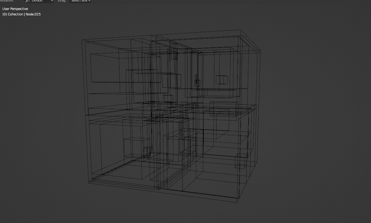
After we have completed these steps, this is the resulting model. Already it’s easier to get an idea how the structure partitions the scene but without the primitives, we don’t have the full picture of what’s going on here yet.
Just like the bounding box points, we can output these to a file and import them as a final step. A quick way to export the triangles from the raytracing application is to use the STL format, which can be seen below. For this demonstration, I will only be using flat shading so we can skip the normals of the primitives.
solid Triangles_output
  facet normal 0 0 0
    outer loop
      vertex -2.46422 -4.2492 -0.232984
      vertex -2.30149 -3.81082 0.273664
      vertex -1.63817 -3.4793 0.30526
    endloop
  endfacet
endsolid
Of course, there will be plenty more triangles in the actual file but you get the idea. With the STL file written, we can now import it to Blender and see the full picture of the structure:
In summary, this was the quickest way I could think out to visualize the BVH acceleration structure when I started implementing it for Luz. Over time, this will be integrated as a separate feature into Luz once my implementation has been proved to work for more complicated scenes than just a few single textured meshes as demonstrated in my alpha demo video from last month.
Live long and prosper!
Another Luz raytracer update, this time I have implemented textured meshes and depth of field along with better image accumulation improving image quality over time. In order to speed up swapping between scenes, I also ended up creating a custom file browser in ImGui which does the job for now.
I haven’t really decided on the logo yet but I’ve started to look into the aesthetics of the application, hopefully I will be able to come up with some good color palette in the future to give it a bit more personality.
To celebrate the progress of this project, I decided to recreate the test scene from Ray Tracing in One Weekend which is another great book I’ve taken a lot of inspiration from while implementing Luz.
Enjoy! 🙂

Back again with a showcase of my new raytracer called Luz, simply meaning “light” in Spanish 🙂
It currently only supports CPU rendering BUT, with the additional options of tiled rendering and multithreading. I have plans for this summer vacation to integrate last year’s Vulkan backend to allow for the more efficient GPU rendering alternative, but there’s still some fundamental work left on the GUI before I’ll take that step.
Mesh intersection is also further optimized using bounding volume hierarchies, in which I started off with a naive implementation based on the book “An Introduction to Raytracing”. It’s a bit dated but most of the math is still relevant to this day and essentially all modern raytracing builds upon the practices discussed in this book. Highly recommended!
The goal of the tool is to make it easier for myself to develop new raytracing features and also speed up the learning process by making the entire experience more interactive – which was exactly what I was lacking in the Vulkan raytracer prototype. With the help of Luz, I might hopefully be able to take on more challenging tasks that was beyond my reach only a year ago.
There’s also been plenty of mistakes along the way as well for both the CPU and GPU approach, even for some of the minor image corrections. I hope to find the time to discuss this in some future posts when I can compile my notes into something that’s actually readable along with the source code which will be uploaded to Github when the project has matured a bit.
Until then, take care and have a wonderful summer!

In January this year, I decided to take the time and learn the Vulkan API as a competency development initiative at work. The first thing I’ve successfully implemented using my raytracer is the classic Cornell Box scene, which you can see a short demo about in the video below:
This has been a huge personal milestone to me as a graphics programmer and one of the most exciting projects I’ve ever worked on during my free time. After all, I’m still learning as I go along and revisiting the intersection tests that I learnt at university has been a good practice to reflect on some of the concepts that I couldn’t quite grasp a few years ago. I would like to extend a special thanks to my friend Jonathan Carrera who helped me review some of these intersection tests during my vacation and got me up to speed again with the mathematics behind the algorithms.
However, you can probably notice from the demo that I’m currently struggling a bit with noise in the output image and haven’t really been able to find the optimal settings yet to produce cleaner images. Well, that’s next on the agenda! This is only the start of a great adventure for me and I’m looking forward to continue playing around with this project and improving on it for the rest of the year.
Stay tuned, I’ll keep posting videos of my project in the future when the next demo is ready. Stay safe 🙂