Since I just learned to play most parts of the song Stinkfist and recorded it in one of my sessions, I wanted to accompany that with a short animation in true TOOL fashion. This was a quick effect I threw together but I thought it would be fun just to cover some of the highlights in the process.
Process
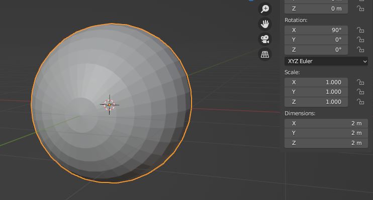
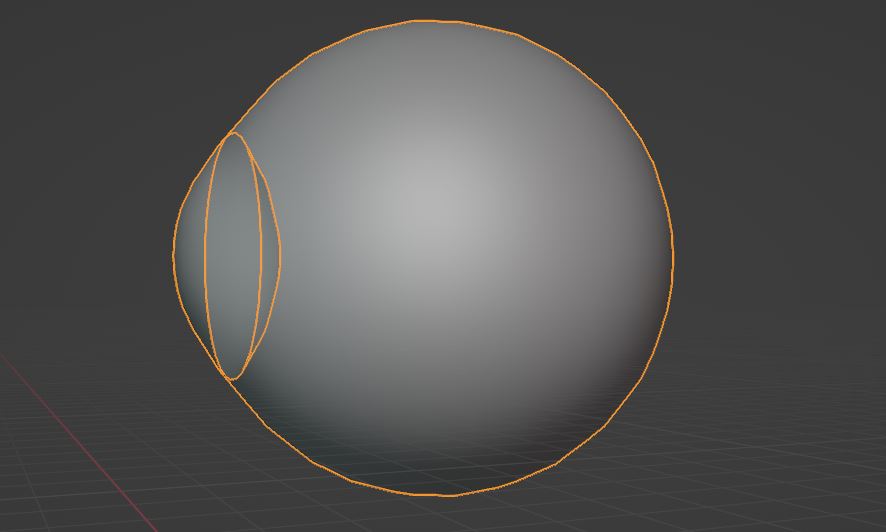
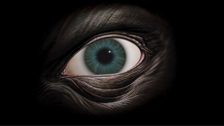
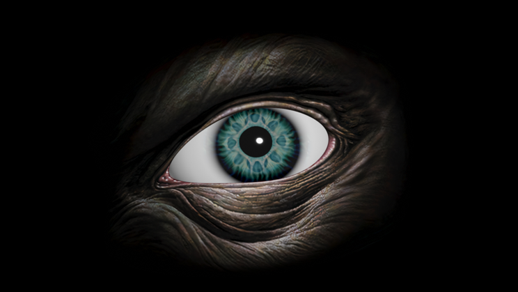
The UV sphere is a good starting mesh but we have to remember that eyes aren’t perfectly round so we need to take that into account. The edges at the pole create rendering artifacts as well, so I remove its geometry and insert another sphere to use as reference when I’m scaling a subdivided surface onto the opening of the eye. Then the backfaces inside of that reference sphere can be be positioned appropriately to function as the iris.
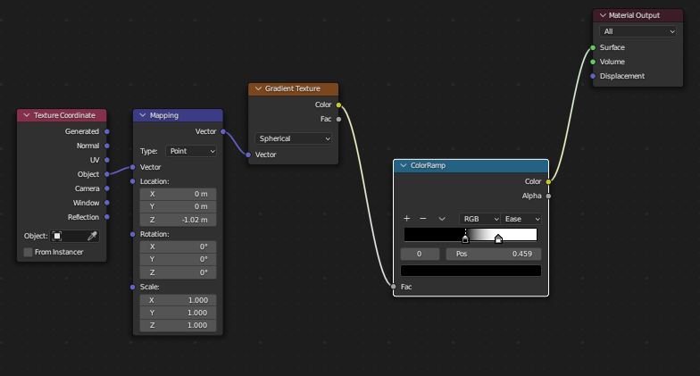
Making procedural eyes in Blender relies heavily on the usage of spherical gradient maps, in which you create masks to form the iris and its various color gradients. The masks are also used to turn off any other effects that overlap with the iris, such as blood vessels which can be created using Voronoi texture nodes.
Just to give you an idea of the underlying shader pipeline, this is what it will look like for most of the time. Lots of masks stacked on top of each other and mixed to combine various effects.
Note that in order to actually be able to make it transparent, we have to enable screen space refractions in the material properties or otherwise this approach won’t work.
From here on, I start modelling an eye socket using the reference image and make sure I’ll capture the general shape of the grooves since they are an important detail.
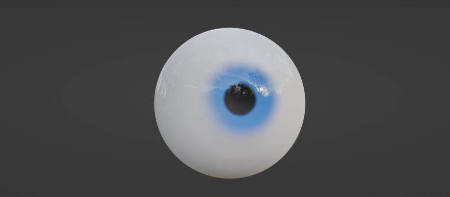
I let Blender solve the UV-mapping for me and I barely had to make any adjustment to the automatic unwrap, this is a nice thing with open meshes that are only viewed from one direction. With the model for the eye socket ready, I’m going to project the original image onto the mesh to get my final texture. Here I’m also starting to make use of the Voronoi Texture to simulate the pigmented layer at the front of our eyes.
On top of this, I also mix in some of the original iris from the painting.
To give the eye a bit more life, I’m going to insert a small amount of morphing on the eyelids using a shape key.
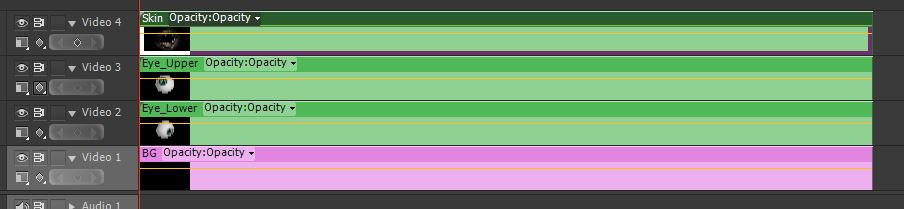
In order to overlap the eyes with as little visual artifacts as possible, I essentially split up each mesh into its separate rendering layer and made a composition of them later in Adobe Premiere.
I settled for a gentle swaying pattern for the camera to make it a bit more haunting and a bit of noise to set the mood, it also helped to blur out the edges of the mesh.
Summary
Below you can see the rendered sequence that I used for my Stinkfist cover, I don’t know about my guitar techniques but I had a lot of fun doing this. I’m thinking about turning this into a series and make a new effect for each TOOL song I learn but that’s yet to come.
Today I’m going to return to the subject of attractors which I started exploring a while back on this page and see if I can come up with some new implementations that I haven’t tried out before. If you want to read about my initial exploration of the Clifford Attractors, you can find it here: Luz: Clifford Attractors Plugin
The reason I was drawn to attractors in the first place is that with a relatively small effort, you can come up with an amazing piece of abstract art that takes on a life of its own in front of your eyes. I will use Unreal Engine 5 to demonstrate how an attractor system can be implemented in Niagara and also expanded to allow the implementation of different attractor solutions.
The Concept of Strange Attractors
Besides being algebraically represented, strange attractors can be treated like just any other particle system (a physical system) where we have starting conditions and a system that evolves over time.
There are many mathematical explanations to what attractors are but the most straightforward way to look at it (the way I look at it I should say) is points within a shape or region that is being pulled around by a set of initial conditions and the systems acting upon these conditions. When I say system, I refer to the system of equations that simulates the behaviors of natural phenomena such as weather. These equations are non-linear, meaning they don’t have a predictable outcome and therefore these attractors falls into the subject of “chaos theory”. For example, two points on the attractor that are near each other at one time can be far apart at later times, resulting in various trajectories.
So if you’ve ever stopped and witnessed a whirlwind of leaves in the fall circling in various patterns, or perhaps observed clouds taking on different formations over time when you’re lying in the grass on a warm summer day, this is essentially the same what we are trying to accomplish with attractors. Fittingly, the first example of a strange attractor was the Lorenz attractor which is based in a mathematical model of the atmosphere. So these behaviors that I mentioned, they are often determined by natural laws such as the laws of fluid dynamics, which is the case for the Lorenz attractor.
What does this mean for us as visual artists? Well, we can utilize these concepts to follow the trajectories of the points in the system and visualize them with shaders! The implementation we are making today is a Dequan Li attractor, which is a modification of the Lorenz system.
Setting Up The Source Emitter
For this implementation, we want to start out with a complete blank scene.
File > New Level > Empty Level
Next, we need to create a Niagara system.
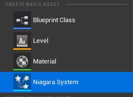
Right-click in the workspace > Create Basic Asset> Niagara System
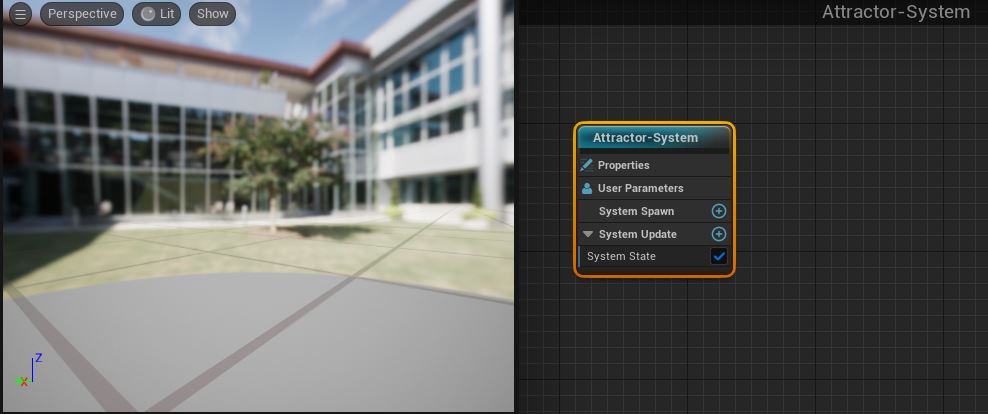
When we double-click the Niagara System we created, we will open up the editor for the simulation.
The environment background will be somewhat distracting so in order to remove it, you must head over the the preview settings in the Windows tab.
Window > Preview Scene Settings > Environment > Show Environment
To start off our implementation, create a new empty emitter which we are going to use as our “source” for the system
Turn on local space for the emitter and set the loop duration mode to infinite. Local space makes sure that the particles spawned by this emitter is relative to the emitter origin.
Loop the particle lifetime in the particle state
Add a scratch pad module to the particle state, which we will use to implement the main logic of the particle update
With the scratch pad module, we’re approaching it like a regular shader pipeline where we will gather inputs in the form of a buffer (Map Get node). In the Map Get node, we will create float variables for the different constants that are commonly found in the equations.
We also create a position variable which we will later on feed with the current position of each particle.
Next we create an custom HLSL node (High-level shader language) which we will attach our inputs to and also define the output.
The output from this stage will be the new position of the particle and this will be directed to the “Velocity” attribute of particle system.
Before we get into writing the shader, I’m going to hook up the input parameters to the shader with user defined fields so that we can quickly change the constants from the main editor without having to open the particle system every time we want to change them.
Next one is important because now we must direct the particle position to the shader “position” input parameter, otherwise we won’t be able to modify the particle position.
Rendering the Attractor
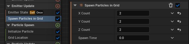
To actually make the particles appear, we need to add “Spawn Particles in Grid” underneath the “Emitter Update”.
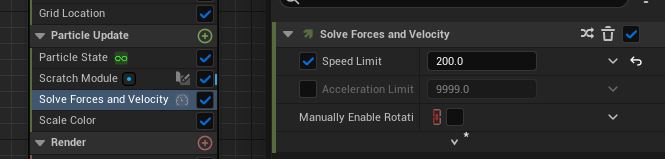
If you ever need to constrain the speed of your particles and I would recommend having this on regardless, you can control this in “Solve Forces and Velocity” underneath the “Particle Update” category.
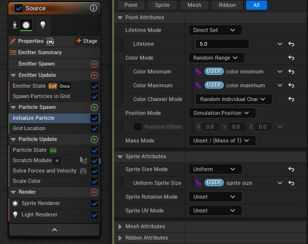
We can also setup a color range in the “Particle Spawn” category using our exposed user variables to give the attractor a gradient look. With the sprite render enabled as well, we can also expose control of the sprite size.
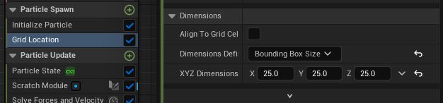
Also, make sure to set an appropriate boundary between the particles in order to not have them bleed into each other.
From here on, it’s possible to use this emitter as a base for other emitters by allowing them to sample the “Source” emitter and extend its behaviors, or even attach additional rendering options onto it. As you can see below, I have chained together the particle system with two renderers; one sprite renderer attached on the “Source” emitter and a ribbon renderer attached onto a second emitter.
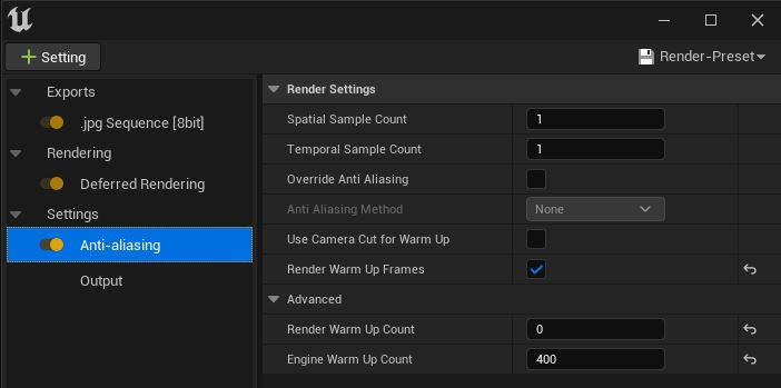
There is a final detail I would like to mention that is useful when exporting rendered sequences of particle systems in Unreal Engine and that is utilizing the warmup settings in the particle system properties. Depending on how you want to capture your particle system, whether it is using an orbital camera or a custom defined path, it might take some time before the attractor has evolved enough so that the points are separated enough that it will fill up most of the frame. In order to not waste any frames and skip forward into the simulation, we set a warmup timer in seconds.
You might only notice this effect in the preview window of your particle system but you will also see this in effect when you are rendering the sequence if you’ve added warmup frames in your render config as well. I’m not certain why this option is hidden underneath the “Anti-Aliasing” setting but there you have it.
During export, you will see this status in the lower right corner indicating that the engine is still warming up. Once the amount of frames that were specified has been reached, the renderer will start to export the images to disk.
Dequan Li shader implementation
With all those preparations made, we can now translate the Dequan Li equations to a HLSL shader code below:
out_position = position;
float x = position.x;
float y = position.y;
float z = position.z;

float dx = alpha * (y-x) + delta * x * z;
float dy = rho * x + zeta * y - x * z;
float dz = beta * z + x * y - epsilon * pow(x, 2);

out_position += vec3(dx, dy, dz);
Summary
This was a quick overview of how the Niagara system in Unreal Engine 5 can be used to visualize strange attractors using a HLSL shader approach. Below you can see the rendered sequence in action where I have used a scaled up Dequan Li attractor that I produced for this post:
Recently I’ve been working on a lot of small projects in Maya during my free time, with this being one of the most challenging one. It’s a work in progress of my Fluid Dynamics experiments, in which my goal is to learn more about Maya’s fluid & particle simulations in order to create better visual effects. I’m going to try everything from making realistic fire and weather effects but for now I’m just focusing on the tornado.
So far so good, but I’m probably going to make a new blend between my cached animations. I’m not really where I want to be yet, but eventually I’ll get there. Enjoy 🙂